How to Separate First and Last Names in Excel

We'll show you how to set up your own formula

Written by: Aseem Kishore, Twitter: @akishore
Posted on: March 19th, 2018 in: MS Office Tips

If you use Excel a lot, you have probably run across a situation where you have a name in a single cell and you need to separate the name into different cells. This is a very common issue in Excel and you can probably do a Google search and download 100 different macros written by various people to do it for you.

However, in this post, I’ll show you how to setup a formula so you can do it yourself and actually understand what is going on. If you use Excel a lot, it’s probably a good idea to learn some of the more advanced functions so that you can do more interesting things with your data.

Table of Contents

If you don’t like formulas and want a quicker solution, scroll down to the Text to Columns section, which teaches you how to use an Excel feature to do the same thing. In addition, the text to columns feature is also better to use if you have more than two items in a cell you need to separate. For example, if one column has 6 fields combined together, then using the formulas below will become really messy and complicated.

Separate Names in Excel

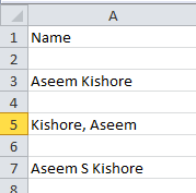
To get started, let’s see how names are usually stored in a Excel spreadsheet. The most common two ways I have seen are firstname lastname with just a space and lastname, firstname with a comma separating the two. Whenever I have seen a middle initial, it’s usually firstname midinitial lastname like below:

Using some simple formulas and combining a couple of them together, you can easily separate the first name, last name and middle initial into separate cells in Excel. Let’s start with extracting the first part of the name. In my case, we’re going to use two functions: left and search. Logically here’s what we need to do:

Search the text in the cell for a space or comma, find the position and then take out all the letters to the left of that position.

Here’s a simple formula that gets the job done correctly: =LEFT(NN, SEARCH(” “, NN) – 1), where NN is the cell that has the name stored in it. The -1 is there to remove the extra space or comma at the end of the string.

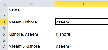
As you can see, we start out with the left function, which takes two arguments: the string and the number of characters you want to grab starting from the beginning of the string. In the first case, we search for a space by using double quotes and putting a space in-between. In the second case, we are looking for a comma instead of a space. So what is the result for the 3 scenarios I have mentioned?

We got the first name from row 3, the last name from row 5 and the first name from row 7. Great! So depending on how your data is stored, you have now extracted either the first name or the last name. Now for the next part. Here’s what we need to do logically now:

– Search the text in the cell for a space or comma, find the position and then subtract the position from total length of the string. Here’s what the formula would look like:

=RIGHT(NN,LEN(NN) -SEARCH(” “,NN))

So now we use the right function. This takes two arguments also: the string and the number of characters you want to grab starting from the end of the string going left. So we want the length of the string minus the position of the space or comma. That will give us everything to the right of the first space or comma.

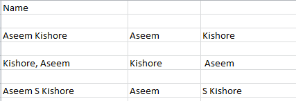
Great, now we have the second part of the name! In the first two cases, you’re pretty much done, but if there is a middle initial in the name, you can see that the result still includes the last name with the middle initial. So how do we just get the last name and get rid of the middle initial? Easy! Just run the same formula again that we used to get the second section of the name.

So we are just doing another right and this time applying the formula on the combined middle initial and last name cell. It will find the space after the middle initial and then take the length minus the position of the space number of characters off the end of the string.

So there you have it! You have now split the first name and last name into separate columns using a few simple formulas in Excel! Obviously, not everyone will have their text formatted in this way, but you can easily edit it to suit your needs.

Text to Columns

There is also another easy way you can separate combined text into separate columns in Excel. It’s a featured called Text to Columns and it works very well. It’s also much more efficient if you have a column that has more than two pieces of data.

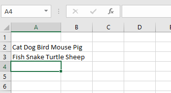
For example, below I have some data where one row has 4 pieces of data and the other row has 5 pieces of data. I would like to split that into 4 columns and 5 columns, respectively. As you can see, trying to use the formulas above would be impractical.

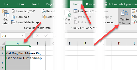
In Excel, first select the column you want to separate. Then, go ahead and click on the Data tab and then click on Text to Columns.

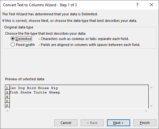
This will bring up the Text to Columns wizard. In step 1, you choose whether the field is delimited or fixed width. In our case, we’ll choose Delimited.

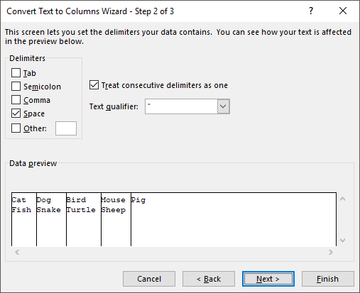
On the next screen, you will choose the delimiter. You can pick from tab, semicolon, comma, space or type a custom one in.

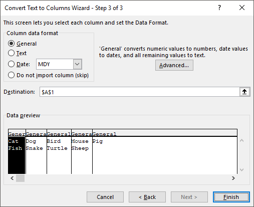
Finally, you choose the data format for the column. Normally, General will work just fine for most types of data. If you have something specific like dates, then choose that format.

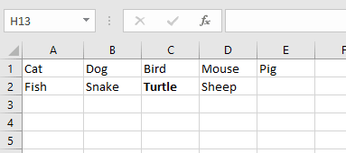
Click Finish and watch how your data is magically separated into columns. As you can see, one row turned into five columns and the other one into four columns. The Text to Columns feature is very powerful and can make your life a lot easier.